Simulating observations with MUSTANG-2
MUSTANG-2 is a bolometric array on the Green Bank Telescope. In this notebook we simulate an observation of a galactic cluster.
[1]:
import maria
map_filename = maria.io.fetch("maps/small_cluster.h5")
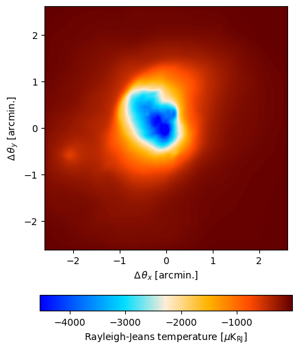
input_map = maria.map.load(
nu=930e9,
filename=map_filename, # filename
width=6/60, # width in degrees
center=(144, 12), # position in the sky
frame="ra_dec",
units="Jy/pixel", # units of the input map
)
input_map.plot()
Downloading https://github.com/thomaswmorris/maria-data/raw/master/maps/small_cluster.h5: 100%|██████████| 3.45M/3.45M [00:00<00:00, 155MB/s]
[2]:
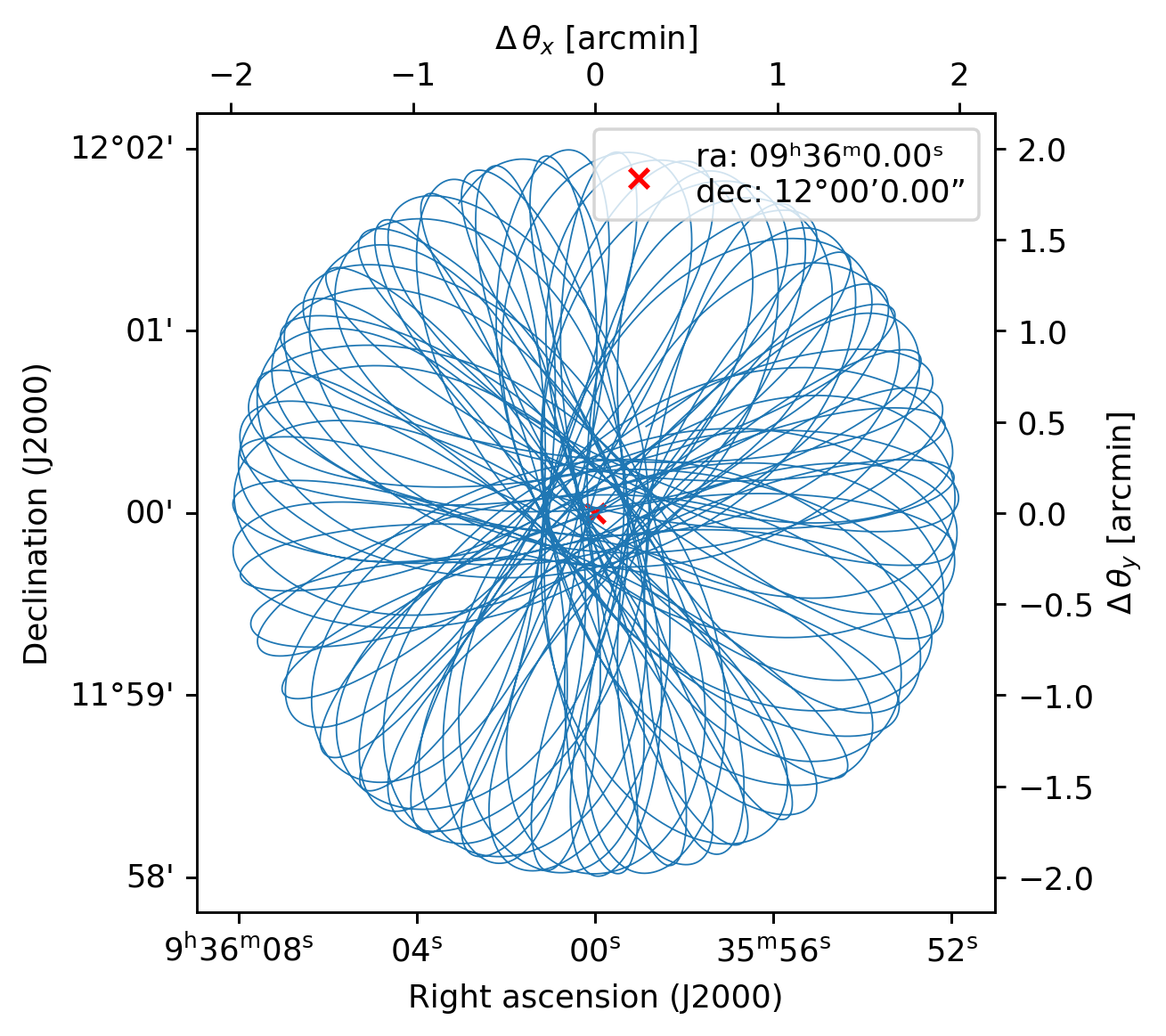
plan = maria.get_plan(
    scan_pattern="daisy",  # scanning pattern
    scan_options={"radius": 2/60, "speed": 0.5/60},  # in degrees
    duration=1200,  # integration time in seconds
    sample_rate=50,  # in Hz
    scan_center=(144, 12),  # position in the sky
    frame="ra_dec",
)

plan.plot()
[3]:
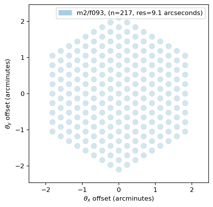
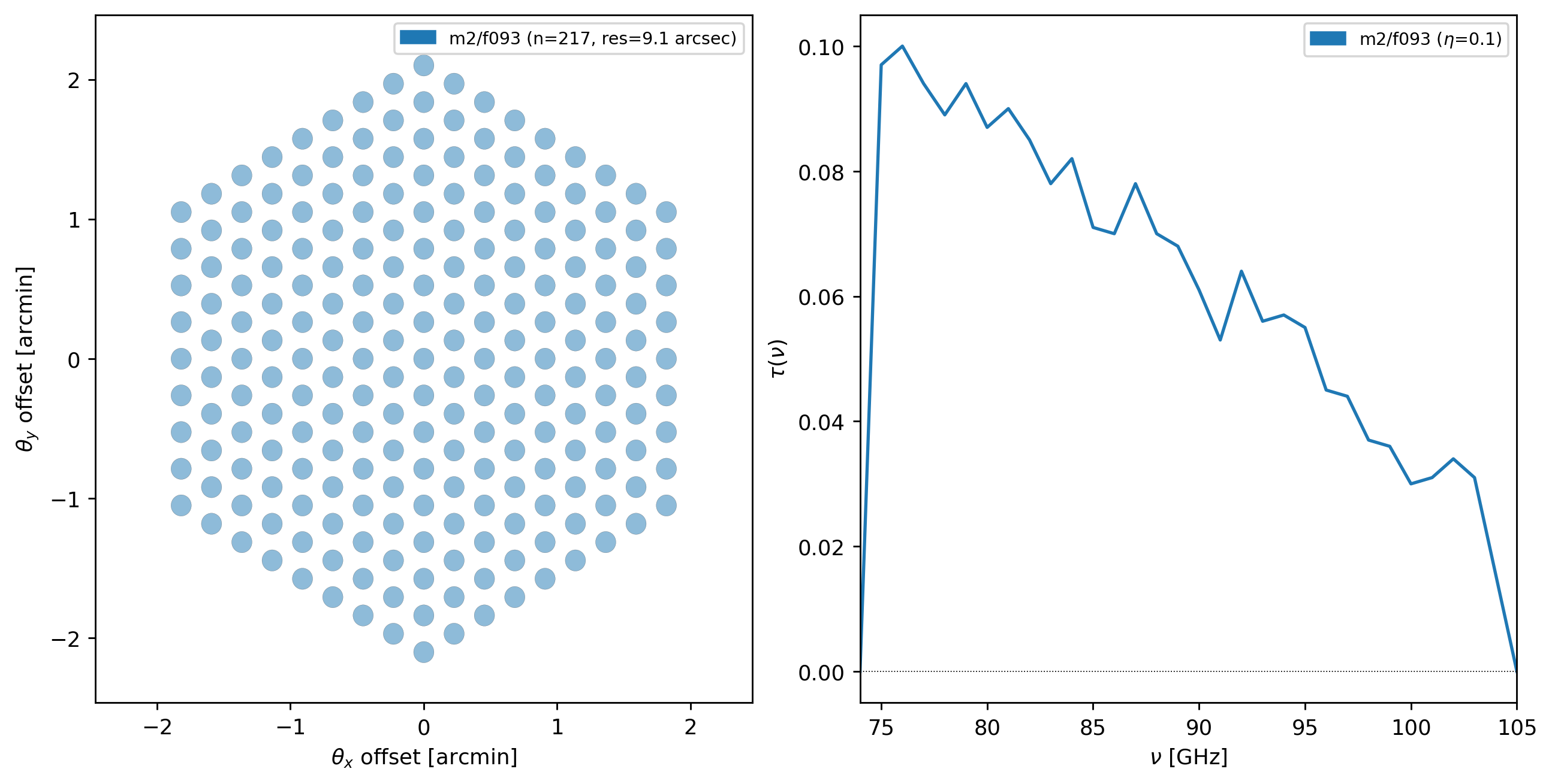
instrument = maria.get_instrument("MUSTANG-2")
print(instrument)
instrument.plot()
Instrument(1 array)
├ arrays:
│            n         FOV baseline      bands
│  array1  217  4.2 arcmin      0 m  [m2/f093]
│
└ bands:
               center      width    η      NEP      NET_RJ     NET_CMB  \
   m2/f093  86.21 GHz  20.98 GHz  0.1  30 aW√s  1.142 mK√s  1.381 mK√s

                    FWHM
   m2/f093  9.133 arcsec
[4]:
sim = maria.Simulation(
    instrument,
    plan=plan,
    site="green_bank",
    map=input_map,
    atmosphere="2d",
)

print(sim)
Downloading https://github.com/thomaswmorris/maria-data/raw/master/atmosphere/spectra/am/v2/green_bank.h5: 100%|██████████| 11.1M/11.1M [00:00<00:00, 201MB/s]
Downloading https://github.com/thomaswmorris/maria-data/raw/master/atmosphere/weather/era5/green_bank.h5: 100%|██████████| 12.0M/12.0M [00:00<00:00, 175MB/s]
Constructing atmosphere: 100%|██████████| 6/6 [00:07<00:00,  1.28s/it]
Simulation
├ Instrument(1 array)
│ ├ arrays:
│ │            n         FOV baseline      bands
│ │  array1  217  4.2 arcmin      0 m  [m2/f093]
│ │
│ └ bands:
│                center      width    η      NEP      NET_RJ     NET_CMB  \
│    m2/f093  86.21 GHz  20.98 GHz  0.1  30 aW√s  1.142 mK√s  1.381 mK√s
│
│                     FWHM
│    m2/f093  9.133 arcsec
├ Site:
│   region: green_bank
│   location: 38°25’59.16”N 79°50’23.28”W
│   altitude: 0.825 km
│   seasonal: True
│   diurnal: True
├ Plan:
│   start_time: 2024-02-10 06:00:00.000 +00:00
│   duration: 1200 s
│   sample_rate: 50 Hz
│   center:
│     ra: 09ʰ36ᵐ0.00ˢ
│     dec: 12°00’0.00”
│   scan_pattern: daisy
│   scan_radius: 4 arcmin
│   scan_kwargs: {'radius': 0.03333333333333333, 'speed': 0.008333333333333333}
├ Atmosphere(6 processes with 6 layers):
│ ├ spectrum:
│ │   region: green_bank
│ └ weather:
│     region: green_bank
│     altitude: 0.825 km
│     time: Feb 10 01:09:59 -05:00
│     pwv[mean, rms]: (8.097 mm, 242.9 um)
└ ProjectedMap:
    shape[stokes, nu, t, y, x]: (1, 1, 1, 1000, 1000)
    stokes: ['I']
    nu: [0.93] THz
    t: [1.74501855e+09] s
    quantity: rayleigh_jeans_temperature
    units: K_RJ
      min: -1.831e-02
      max: -1.746e-05
    center:
      ra: 09ʰ36ᵐ0.00ˢ
      dec: 12°00’0.00”
    size[y, x]: (6 arcmin, 6 arcmin)
    resolution[y, x]: (360 marcsec, 360 marcsec)
    memory: 8 MB
[5]:
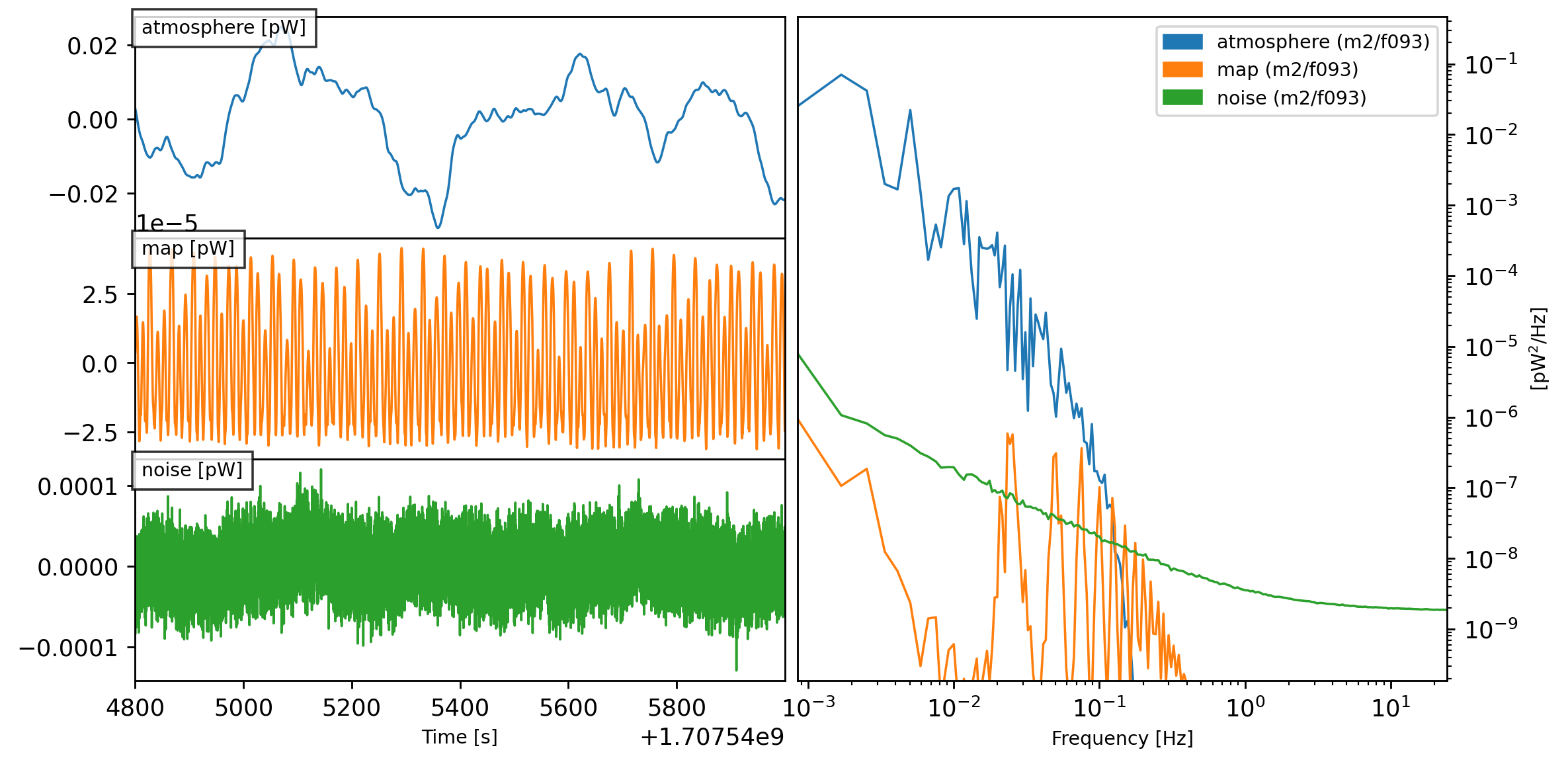
tod = sim.run()
tod.plot()
Generating turbulence: 100%|██████████| 6/6 [00:00<00:00, 30.26it/s]
Sampling turbulence: 100%|██████████| 6/6 [00:01<00:00,  3.57it/s]
Computing atmospheric emission: 100%|██████████| 1/1 [00:02<00:00,  2.13s/it, band=m2/f093]
Sampling map: 100%|██████████| 1/1 [00:03<00:00,  3.97s/it, band=m2/f093]
Generating noise: 100%|██████████| 1/1 [00:00<00:00,  1.05it/s, band=m2/f093]
[6]:
from maria.mappers import BinMapper

mapper = BinMapper(
    center=(144, 12),
    frame="ra_dec",
    width=6/60,
    height=6/60,
    resolution=0.03/60,
    tod_preprocessing={
        "window": {"name": "hamming"},
        "remove_modes": {"modes_to_remove": [0]},
        "remove_spline": {"knot_spacing": 30, "remove_el_gradient": True},
    },
    map_postprocessing={
        "gaussian_filter": {"sigma": 1},
        "median_filter": {"size": 1},
    },
    units="uK_RJ",
)

mapper.add_tods(tod)
output_map = mapper.run()
2025-04-22 16:17:45.387 INFO: Ran mapper for band m2/f093 in 12.73 s.
[7]:
output_map.plot()
output_map.to_fits("/tmp/simulated_mustang_map.fits")