Custom map simulations
In this tutorial we will build a simulation from scratch.
We start by defining a Band that will determine our array’s sensitivity to different spectra. We then generate an array by specifying a field of view, which will be populated by evenly-spaced beams of the given band.
[1]:
import maria
from maria.instrument import Band
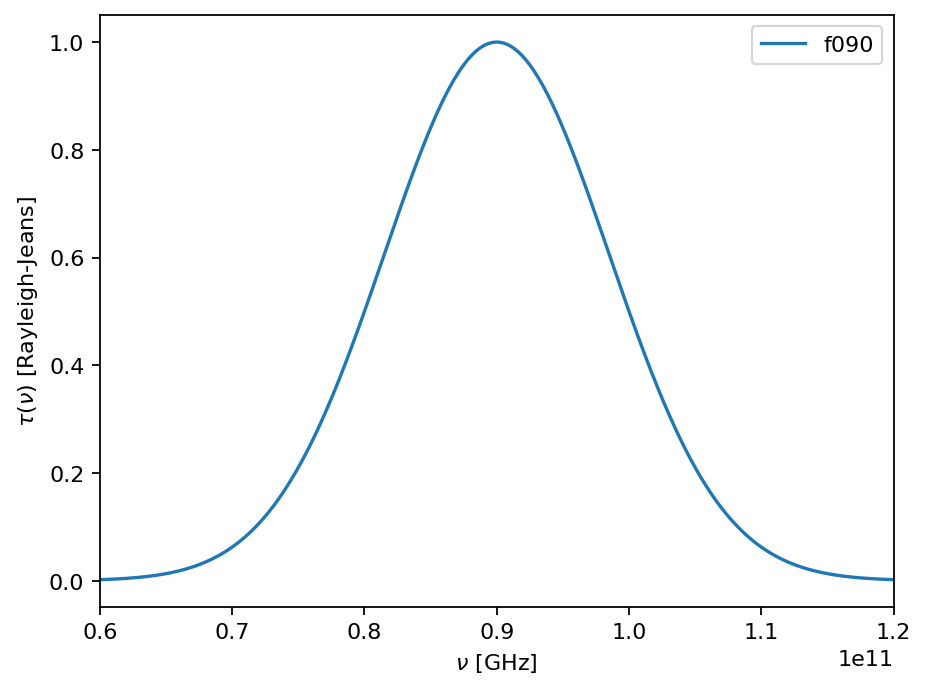
f090 = Band(
center=90e9, # in Hz
width=20e9, # in Hz
NET_RJ=40e-6, # in K sqrt(s)
knee=1e0, # in Hz
gain_error=5e-2)
f150 = Band(
center=150e9,
width=30e9,
NET_RJ=60e-6,
knee=1e0,
gain_error=5e-2)
f090.plot()
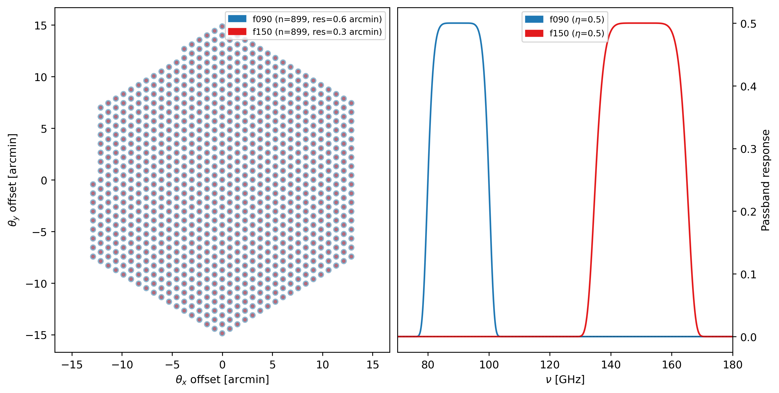
We next define an array config, which specifies how detectors will be distributed on the focal plane. In this case, we supply our two bands as the bands argument, which will generate an array of multichroic detectors (for monochroic detectors, we would supply e.g. "bands": [f090]). The resolution of each detector is determined by frequency of the band and the primary_size parameter. The number of detectors is determined by filling up the specified field_of_view with detector
beams, with a relative spacing determined by the beam_spacing parameter.
[2]:
array = {"field_of_view": 0.1,
         "beam_spacing": 1.5,
         "primary_size": 50,
         "bands": [f090, f150]}

instrument = maria.get_instrument(array=array)

print(instrument)
instrument.plot()
Instrument(1 array)
├ arrays:
│            n field_of_view max_baseline        bands polarized primary_size
│  array1  328        6.124’          0 m  [f090,f150]     False         50 m
│
└ bands:
      name   center   width    η         NEP      NET_RJ         NET_CMB   FWHM
   0  f090   90 GHz  20 GHz  0.5  5.876 aW√s  40 uK_RJ√s  49.15 uK_CMB√s  17.5”
   1  f150  150 GHz  30 GHz  0.5  13.22 aW√s  60 uK_RJ√s    104 uK_CMB√s  10.5”
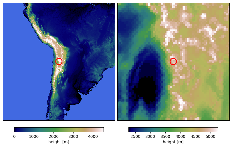
The Site defines the observing location, as well as the weather conditions. maria knows about a bunch of astronomical observing sites (to see them, run print(maria.site_data)); we can instantiate them using the get_site function. We can modify the site by passing kwargs to the get_site function, like changing its altitude (which will affect the vertical profile of different atmospheric parameters).
[3]:
site = maria.get_site("llano_de_chajnantor", altitude=5065)

print(site)
site.plot()
Site:
  region: chajnantor
  timezone: America/Santiago
  location:
    longitude: 67°45’17.28” W
    latitude:  23°01’45.84” S
    altitude: 5.065 km
  seasonal: True
  diurnal: True
2026-06-05 13:40:58.793 INFO: Fetching https://github.com/thomaswmorris/maria-data/raw/master/world_heightmap.h5
Downloading: 100%|██████████| 7.34M/7.34M [00:00<00:00, 144MB/s]
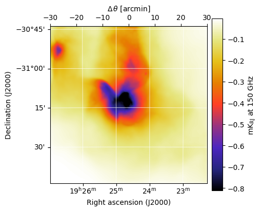
Here the fetch function downloads a map to the path map_filename, but map_filename can be any .h5 or .fits file of an image that corresponds to the maria map convention (see Maps). Additional kwargs added to the maria.map.load overwrite the metadata of the loaded map.
[4]:
from maria.io import fetch

map_filename = fetch("maps/30dor.fits")

input_map = maria.map.load(
    filename=map_filename,
    nu=150e9,
    center=(291.156, -31.23))
input_map.data *= 5e1

print(input_map)
input_map.to("K_RJ").plot()
2026-06-05 13:41:00.347 INFO: Fetching https://github.com/thomaswmorris/maria-data/raw/master/maps/30dor.fits
Downloading: 100%|██████████| 259k/259k [00:00<00:00, 18.0MB/s]
ProjectionMap:
  data(1, 251, 251):
    min: 1.287e+02
    max: 3.473e+04
    units: MJy sr^-1
    quantity: spectral_radiance
  nu(1):
    values: [150.] GHz
  eta(251):
    height: 9’
    res: -2.16”
  xi(251):
    width: 9’
    res: 2.16”
  frame: ra/dec
  center:
    ra: 19ʰ24ᵐ37.44ˢ
    dec: -31°13’48.00”
  beam(maj, min, psi): (0 rad, 0 rad, 0 rad)
  memory: 252 kB
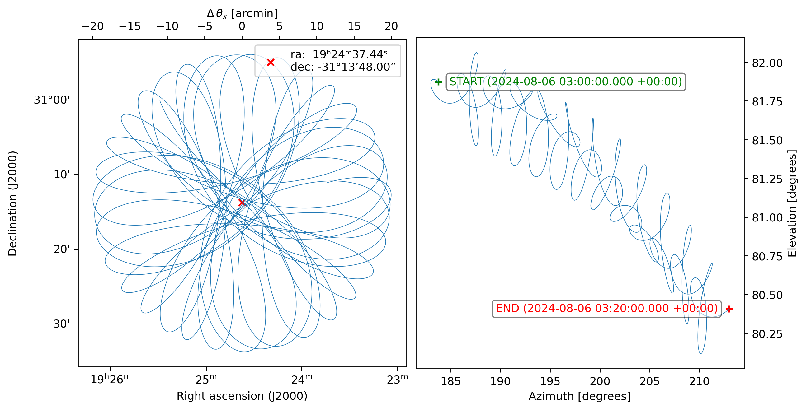
We plan an observation using the Planner, which ensures that a given target as seen by a given site will be high enough above the horizon.
[5]:
from maria import Planner

planner = Planner(start_time="2024-08-06T03:00:00",
                  target=input_map,
                  site=site,
                  constraints={"el": (70, 90)})

plans = planner.generate_plans(total_duration=1200,  # in seconds
                               max_chunk_duration=600,  # in seconds
                               scan_pattern="daisy",
                               scan_options={"radius": input_map.width.deg / 3},
                               sample_rate=10)

print(plans)
plans[0].plot()
PlanList(2 plans, 1200 s):
                           start_time duration     target(ra,dec)     center(az,el)
chunk
0      2024-08-07 01:31:15.000 +00:00    600 s  (291.2°, -31.23°)  (119.7°, 71.13°)
1      2024-08-07 01:41:52.500 +00:00    600 s  (291.2°, -31.23°)  (122.6°, 73.23°)
[6]:
sim = maria.Simulation(
    instrument,
    plans=plans,
    site=site,
    atmosphere="2d",
    atmosphere_kwargs={"weather": {"pwv": 0.5}},
    map=input_map)

print(sim)
2026-06-05 13:41:08.085 INFO: Fetching https://github.com/thomaswmorris/maria-data/raw/master/atmosphere/spectra/am/v3/chajnantor.h5
Downloading: 100%|██████████| 32.9M/32.9M [00:00<00:00, 186MB/s]
2026-06-05 13:41:09.616 INFO: Fetching https://github.com/thomaswmorris/maria-data/raw/master/atmosphere/weather/era5/chajnantor.h5
Downloading: 100%|██████████| 4.05M/4.05M [00:00<00:00, 106MB/s]
Constructing atmosphere: 100%|██████████| 8/8 [00:02<00:00,  2.79it/s]
Constructing atmosphere: 100%|██████████| 8/8 [00:02<00:00,  2.90it/s]
Simulation
├ Instrument(1 array)
│ ├ arrays:
│ │            n field_of_view max_baseline        bands polarized primary_size
│ │  array1  328        6.124’          0 m  [f090,f150]     False         50 m
│ │
│ └ bands:
│       name   center   width    η         NEP      NET_RJ         NET_CMB   FWHM
│    0  f090   90 GHz  20 GHz  0.5  5.876 aW√s  40 uK_RJ√s  49.15 uK_CMB√s  17.5”
│    1  f150  150 GHz  30 GHz  0.5  13.22 aW√s  60 uK_RJ√s    104 uK_CMB√s  10.5”
├ Site:
│   region: chajnantor
│   timezone: America/Santiago
│   location:
│     longitude: 67°45’17.28” W
│     latitude:  23°01’45.84” S
│     altitude: 5.065 km
│   seasonal: True
│   diurnal: True
├ PlanList(2 plans, 1200 s):
│                            start_time duration     target(ra,dec)     center(az,el)
│ chunk
│ 0      2024-08-07 01:31:15.000 +00:00    600 s  (291.2°, -31.23°)  (119.7°, 71.13°)
│ 1      2024-08-07 01:41:52.500 +00:00    600 s  (291.2°, -31.23°)  (122.6°, 73.23°)
├ Atmosphere(8 processes with 8 layers):
│ ├ spectrum:
│ │   region: chajnantor
│ └ weather:
│     region: chajnantor
│     altitude: 5.065 km
│     time: Aug 6 21:36:14 -04:00
│     pwv[mean, rms]: (500 um, 15 um)
└ ProjectionMap:
    data(1, 1, 1, 251, 251):
      min: 1.287e+02
      max: 3.473e+04
      units: MJy sr^-1
      quantity: spectral_radiance
    stokes(1):
      components: ['I']
    nu(1):
      values: [150.] GHz
    t(1):
      values: [1.78066686e+09] s
    eta(251):
      height: 9’
      res: -2.16”
    xi(251):
      width: 9’
      res: 2.16”
    frame: ra/dec
    center:
      ra: 19ʰ24ᵐ37.44ˢ
      dec: -31°13’48.00”
    beam(maj, min, psi): (0 rad, 0 rad, 0 rad)
    memory: 252 kB
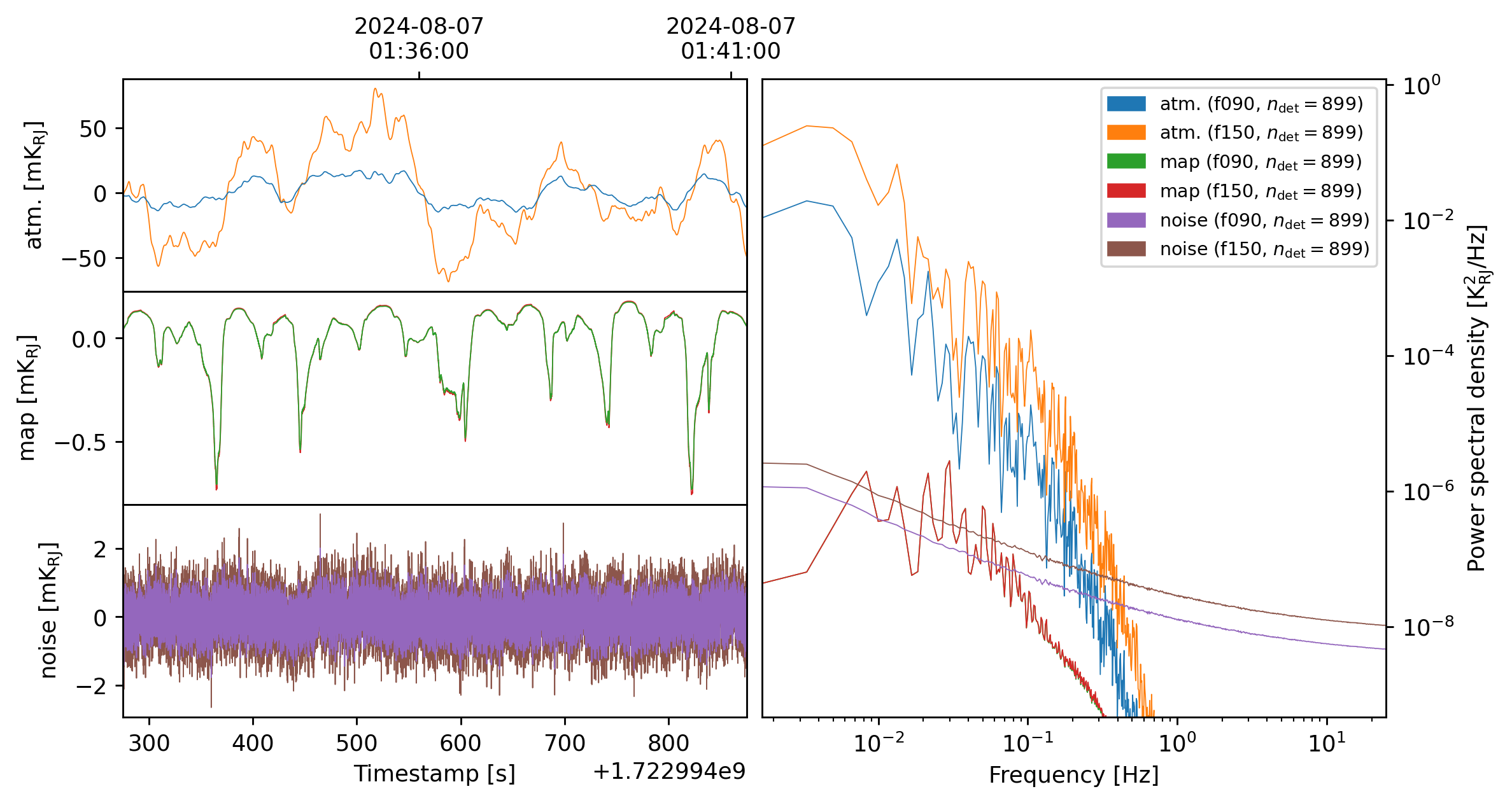
We run the simulation, which spits out a TOD object (which stands for time-ordered data). We can then plot the TOD:
[7]:
tods = sim.run()

print(tods)
tods[0].plot()
2026-06-05 13:41:19.390 INFO: Simulating observation 1 of 2
Generating turbulence: 100%|██████████| 8/8 [00:00<00:00, 18.30it/s]
Sampling turbulence: 100%|██████████| 8/8 [00:04<00:00,  1.85it/s]
Computing atmospheric emission: 100%|██████████| 2/2 [00:02<00:00,  1.02s/it, band=f150]
Sampling map: 100%|██████████| 2/2 [00:03<00:00,  1.64s/it, band=f150, channel=(0 Hz, inf Hz)]
Generating noise: 100%|██████████| 2/2 [00:00<00:00,  2.92it/s, band=f150]
2026-06-05 13:41:32.039 INFO: Simulated observation 1 of 2 in 12.64 s
2026-06-05 13:41:32.040 INFO: Simulating observation 2 of 2
Generating turbulence: 100%|██████████| 8/8 [00:00<00:00, 18.35it/s]
Sampling turbulence: 100%|██████████| 8/8 [00:04<00:00,  1.93it/s]
Computing atmospheric emission: 100%|██████████| 2/2 [00:01<00:00,  1.17it/s, band=f150]
Sampling map: 100%|██████████| 2/2 [00:01<00:00,  1.23it/s, band=f150, channel=(0 Hz, inf Hz)]
Generating noise: 100%|██████████| 2/2 [00:00<00:00,  8.13it/s, band=f150]
2026-06-05 13:41:42.050 INFO: Simulated observation 2 of 2 in 10 s
[TOD(shape=(328, 6000), fields=['atmosphere', 'map', 'noise'], units='K_RJ', start=2024-08-07 01:41:14.899 +00:00, duration=599.9s, sample_rate=10.0Hz, metadata={'atmosphere': True, 'sim_time': <Arrow [2026-06-05T13:41:30.350253+00:00]>, 'altitude': 5065.0, 'region': 'chajnantor', 'pwv': 0.5, 'base_temperature': 272.616, 'input_map': ProjectionMap:
  data(1, 1, 1, 251, 251):
    min: 1.287e+02
    max: 3.473e+04
    units: MJy sr^-1
    quantity: spectral_radiance
  stokes(1):
    components: ['I']
  nu(1):
    values: [150.] GHz
  t(1):
    values: [1.78066686e+09] s
  eta(251):
    height: 9’
    res: -2.16”
  xi(251):
    width: 9’
    res: 2.16”
  frame: ra/dec
  center:
    ra: 19ʰ24ᵐ37.44ˢ
    dec: -31°13’48.00”
  beam(maj, min, psi): (0 rad, 0 rad, 0 rad)
  memory: 252 kB}), TOD(shape=(328, 6000), fields=['atmosphere', 'map', 'noise'], units='K_RJ', start=2024-08-07 01:51:52.399 +00:00, duration=599.9s, sample_rate=10.0Hz, metadata={'atmosphere': True, 'sim_time': <Arrow [2026-06-05T13:41:40.387830+00:00]>, 'altitude': 5065.0, 'region': 'chajnantor', 'pwv': 0.5, 'base_temperature': 272.594, 'input_map': ProjectionMap:
  data(1, 1, 1, 251, 251):
    min: 1.287e+02
    max: 3.473e+04
    units: MJy sr^-1
    quantity: spectral_radiance
  stokes(1):
    components: ['I']
  nu(1):
    values: [150.] GHz
  t(1):
    values: [1.78066686e+09] s
  eta(251):
    height: 9’
    res: -2.16”
  xi(251):
    width: 9’
    res: 2.16”
  frame: ra/dec
  center:
    ra: 19ʰ24ᵐ37.44ˢ
    dec: -31°13’48.00”
  beam(maj, min, psi): (0 rad, 0 rad, 0 rad)
  memory: 252 kB})]
We can then map the TOD using the built-in mapper.
[8]:
from maria.mappers import BinMapper

mapper = BinMapper(
    target=input_map,
    tod_preprocessing={
        "remove_spline": {"knot_spacing": 60, "remove_el_gradient": True},
        "remove_modes": {"modes_to_remove": 1},
    },
    tods=tods,
)

output_map = mapper.run()
2026-06-05 13:41:45.397 INFO: Inferring resolution = 5.249” from detector FWHM
2026-06-05 13:41:45.535 INFO: Inferring stokes parameters 'I' for mapper from detector sensitivities
Preprocessing TODs: 100%|██████████| 2/2 [00:02<00:00,  1.41s/it]
Mapping: 100%|██████████| 2/2 [00:01<00:00,  1.31it/s, tod=1/2]
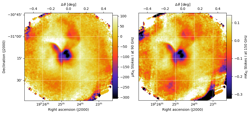
We can see the recovered map with
[9]:
output_map.plot(slices=dict(nu=[0, 1]))
output_map.to_fits("/tmp/output.fits")