Polarized observations
This tutorial covers working with polarized instrument and maps, and recovering polarized maps from observations.
We start with a normal instrument, and create two orthogonally polarized copies of each detector by setting polarized: True in the Array config:
[1]:
import maria
from maria.instrument import Band

f150 = Band(
    center=150e9,
    width=30e9,
    NET_RJ=60e-6,
    knee=1e0,
    gain_error=5e-2)

array = {"field_of_view": 0.2,
         "shape": "circle",
         "beam_spacing": 1.8,
         "primary_size": 10,
         "polarized": True,
         "packing": "sunflower",
         "bands": [f150]}

instrument = maria.get_instrument(array=array)

print(instrument.arrays)
         n field_of_view max_baseline   bands polarized primary_size
array1  88        11.98’          0 m  [f150]      True         10 m
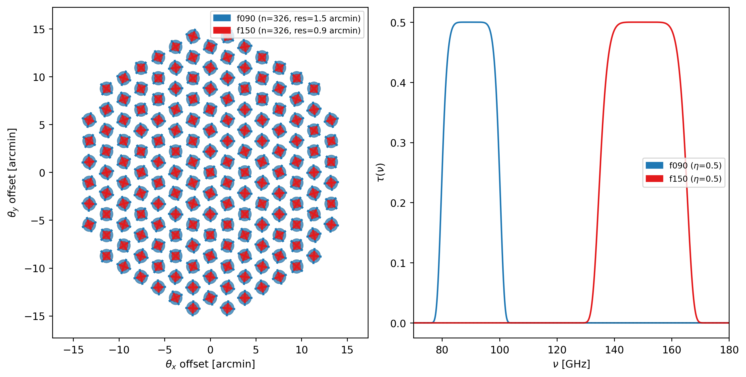
We can see the resulting polarization footprint in the instrument plot:
[2]:
print(instrument)
instrument.plot()
Instrument(1 array)
├ arrays:
│           n field_of_view max_baseline   bands polarized primary_size
│  array1  88        11.98’          0 m  [f150]      True         10 m
│
└ bands:
      name   center   width    η         NEP      NET_RJ       NET_CMB    FWHM
   0  f150  150 GHz  30 GHz  0.5  13.22 aW√s  60 uK_RJ√s  104 uK_CMB√s  52.49”
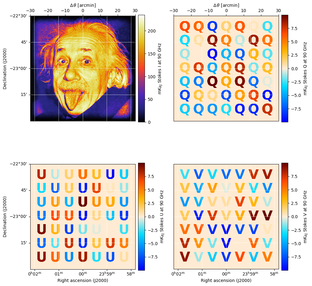
Let’s observe the use the Einstein map, which has a faint polarization signature underneath the unpolarized signal of Einstein’s face. Remember that all maps are five dimensional (stokes, frequency, time, y, x); this map has four channels in the stokes dimensions (the I, Q, U, and V Stokes parameters). We can plot all the channels by giving plot a shaped set of stokes parameters.
[3]:
input_map = maria.map.get("maps/einstein.h5")
input_map.data *= 4
print(input_map)


input_map.plot(slices={"stokes": [["I", "Q"],
                                  ["U", "V"]]})
2026-06-05 13:54:04.764 INFO: Fetching https://github.com/thomaswmorris/maria-data/raw/master/maps/einstein.h5
Downloading: 100%|██████████| 932k/932k [00:00<00:00, 47.6MB/s]
ProjectionMap:
  data(4, 1, 685, 685):
    min: -4.000e-02
    max: 1.016e+00
    units: K_RJ
    quantity: rayleigh_jeans_temperature
  stokes(4):
    components: ['I' 'Q' 'U' 'V']
  nu(1):
    values: [90.] GHz
  eta(685):
    height: 60’
    res: -5.263”
  xi(685):
    width: 60’
    res: 5.263”
  frame: ra/dec
  center:
    ra: 00ʰ00ᵐ0.00ˢ
    dec: -23°00’0.00”
  beam(maj, min, psi): (0 rad, 0 rad, 0 rad)
  memory: 7.508 MB
[4]:
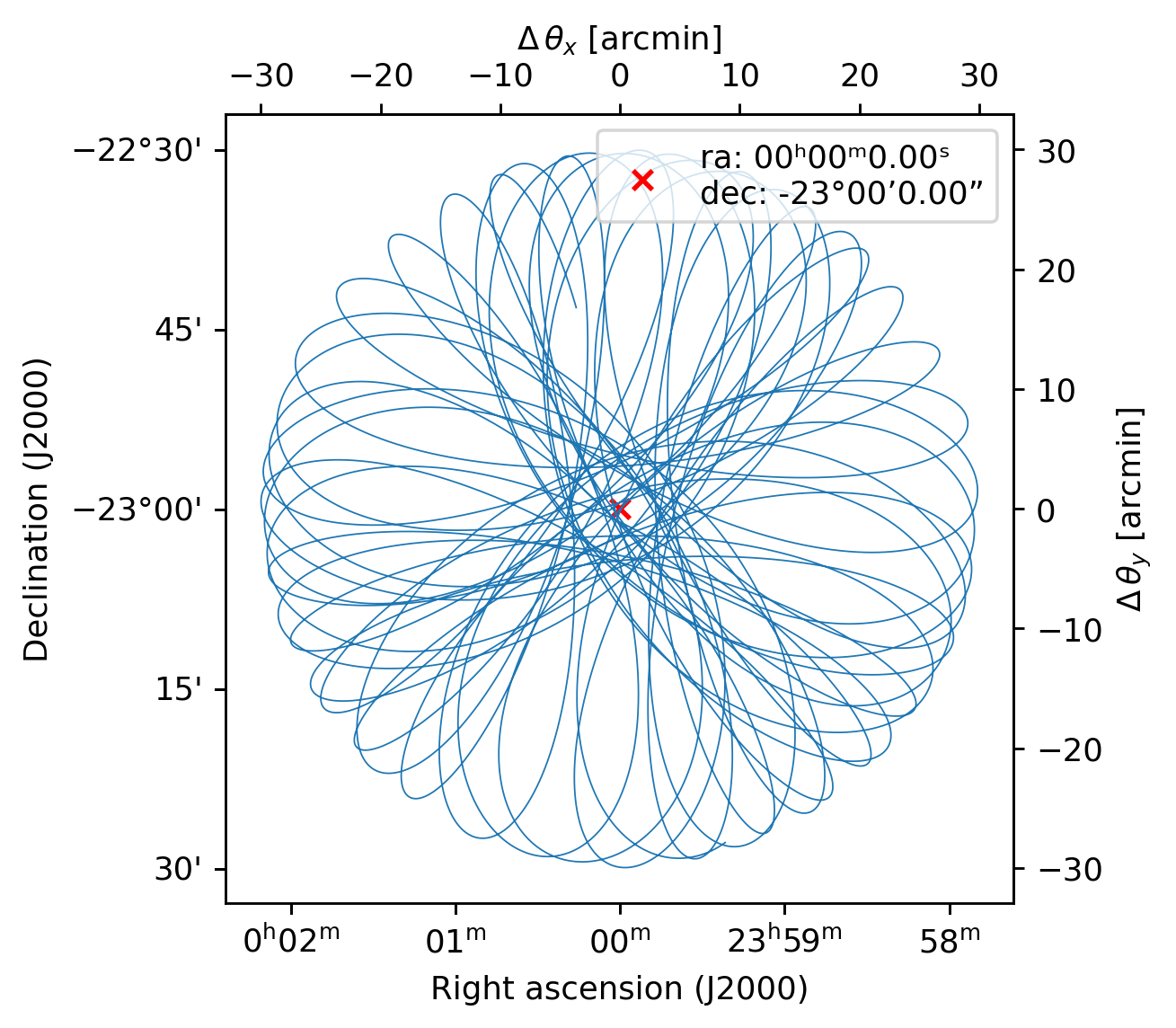
from maria import Planner

planner = Planner(target=input_map, site="mauna_kea", constraints={"el": (45, 90)})

plans = planner.generate_plans(
                               total_duration=1800,
                               max_chunk_duration=1800,
                               sample_rate=50,
                               scan_pattern="raster",
                               scan_options={
                                   "n": [(15, 1), (1, 16)],
                                   "radius": 0.5 * input_map.width.deg,
                                   "speed": 0.5,
                               })

plans[0].plot()
print(plans)
PlanList(1 plans, 1800 s):
                           start_time duration target(ra,dec)  center(az,el)
chunk
0      2026-06-05 16:29:46.491 +00:00   1800 s   (360°, -23°)  (166°, 46.1°)
[5]:
sim = maria.Simulation(
    instrument,
    plans=plans,
    site="mauna_kea",
    atmosphere="2d",
    map=input_map,
)

print(sim)
2026-06-05 13:54:15.558 INFO: Fetching https://github.com/thomaswmorris/maria-data/raw/master/atmosphere/spectra/am/v3/mauna_kea.h5
Downloading: 100%|██████████| 22.0M/22.0M [00:00<00:00, 156MB/s]
2026-06-05 13:54:17.135 INFO: Fetching https://github.com/thomaswmorris/maria-data/raw/master/atmosphere/weather/era5/mauna_kea.h5
Downloading: 100%|██████████| 8.62M/8.62M [00:00<00:00, 126MB/s]
Constructing atmosphere: 100%|██████████| 8/8 [00:47<00:00,  5.89s/it]
Simulation
├ Instrument(1 array)
│ ├ arrays:
│ │           n field_of_view max_baseline   bands polarized primary_size
│ │  array1  88        11.98’          0 m  [f150]      True         10 m
│ │
│ └ bands:
│       name   center   width    η         NEP      NET_RJ       NET_CMB    FWHM
│    0  f150  150 GHz  30 GHz  0.5  13.22 aW√s  60 uK_RJ√s  104 uK_CMB√s  52.49”
├ Site:
│   region: mauna_kea
│   timezone: Pacific/Honolulu
│   location:
│     longitude: 155°28’37.20” W
│     latitude:  19°49’22.08” N
│     altitude: 4.092 km
│   seasonal: True
│   diurnal: True
├ PlanList(1 plans, 1800 s):
│                            start_time duration target(ra,dec)  center(az,el)
│ chunk
│ 0      2026-06-05 16:29:46.491 +00:00   1800 s   (360°, -23°)  (166°, 46.1°)
├ Atmosphere(8 processes with 8 layers):
│ ├ spectrum:
│ │   region: mauna_kea
│ └ weather:
│     region: mauna_kea
│     altitude: 4.092 km
│     time: Jun 5 06:44:46 -10:00
│     pwv[mean, rms]: (2.152 mm, 64.55 um)
└ ProjectionMap:
    data(4, 1, 1, 685, 685):
      min: -4.000e-02
      max: 1.016e+00
      units: K_RJ
      quantity: rayleigh_jeans_temperature
    stokes(4):
      components: ['I' 'Q' 'U' 'V']
    nu(1):
      values: [90.] GHz
    t(1):
      values: [1.78066764e+09] s
    eta(685):
      height: 60’
      res: -5.263”
    xi(685):
      width: 60’
      res: 5.263”
    frame: ra/dec
    center:
      ra: 00ʰ00ᵐ0.00ˢ
      dec: -23°00’0.00”
    beam(maj, min, psi): (0 rad, 0 rad, 0 rad)
    memory: 7.508 MB
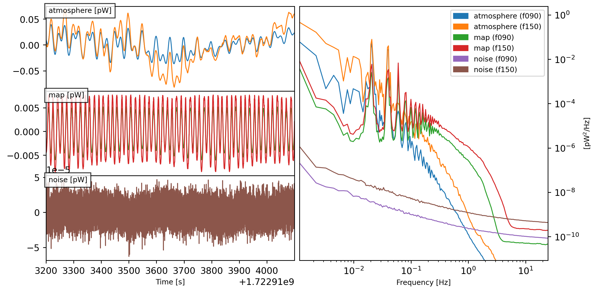
[6]:
tods = sim.run()

print(tods)
tods[0].plot()
2026-06-05 13:55:06.542 INFO: Simulating observation 1 of 1
Generating turbulence: 100%|██████████| 8/8 [00:02<00:00,  3.13it/s]
Sampling turbulence: 100%|██████████| 8/8 [00:05<00:00,  1.47it/s]
Computing atmospheric emission: 100%|██████████| 1/1 [00:01<00:00,  1.38s/it, band=f150]
Sampling map: 100%|██████████| 1/1 [00:04<00:00,  4.79s/it, band=f150, channel=(0 Hz, inf Hz)]
Generating noise: 100%|██████████| 1/1 [00:01<00:00,  1.01s/it, band=f150]
2026-06-05 13:55:26.935 INFO: Simulated observation 1 of 1 in 20.38 s
[TOD(shape=(88, 90000), fields=['atmosphere', 'map', 'noise'], units='K_RJ', start=2026-06-05 16:59:46.469 +00:00, duration=1800.0s, sample_rate=50.0Hz, metadata={'atmosphere': True, 'sim_time': <Arrow [2026-06-05T13:55:22.164513+00:00]>, 'altitude': 4092.0, 'region': 'mauna_kea', 'pwv': 2.152, 'base_temperature': 278.825, 'input_map': ProjectionMap:
  data(4, 1, 1, 685, 685):
    min: -4.000e-02
    max: 1.016e+00
    units: K_RJ
    quantity: rayleigh_jeans_temperature
  stokes(4):
    components: ['I' 'Q' 'U' 'V']
  nu(1):
    values: [90.] GHz
  t(1):
    values: [1.78066764e+09] s
  eta(685):
    height: 60’
    res: -5.263”
  xi(685):
    width: 60’
    res: 5.263”
  frame: ra/dec
  center:
    ra: 00ʰ00ᵐ0.00ˢ
    dec: -23°00’0.00”
  beam(maj, min, psi): (0 rad, 0 rad, 0 rad)
  memory: 7.508 MB})]
[7]:
from maria.mappers import MaximumLikelihoodMapper
mapper = MaximumLikelihoodMapper(
frame="ra/dec",
resolution=2 * input_map.resolution.deg,
tod_preprocessing={
"remove_spline": {"knot_spacing": 300, "remove_el_gradient_order": 1},
},
tods=tods,
bilinear=False,
)
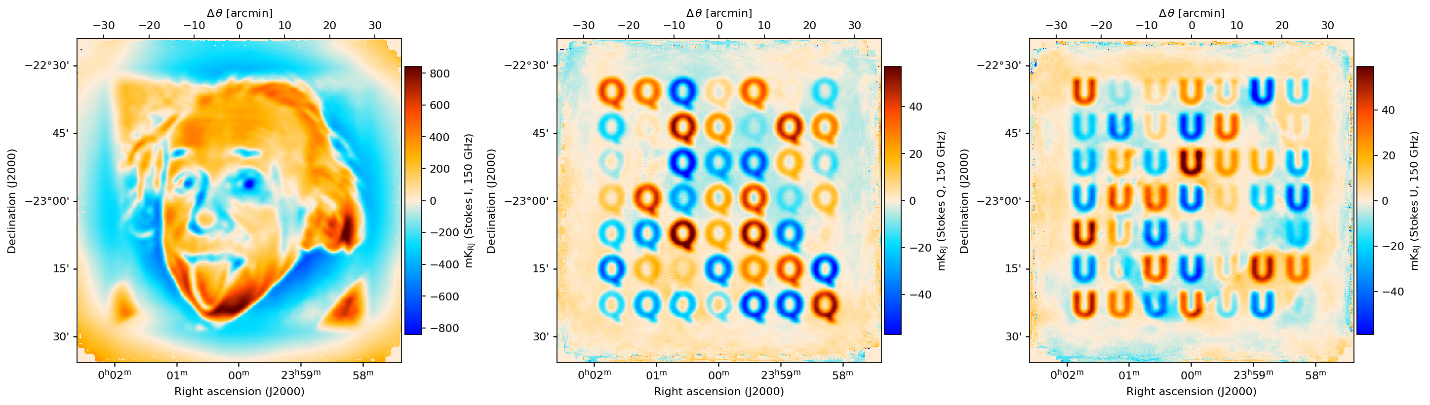
mapper.map.plot(slices="all")
2026-06-05 13:55:32.491 INFO: Inferring center {'ra': '23ʰ59ᵐ59.39ˢ', 'dec': '-22°59’58.10”'} for mapper
2026-06-05 13:55:32.505 INFO: Inferring mapper width 1.198° for mapper from observation patch
2026-06-05 13:55:32.506 INFO: Inferring mapper height 1.198° to match supplied width
2026-06-05 13:55:32.848 INFO: Inferring stokes parameters 'IQU' for mapper from detector sensitivities
Preprocessing TODs: 100%|██████████| 1/1 [00:03<00:00,  3.37s/it]
Computing pointing matrices: 100%|██████████| 1/1 [00:04<00:00,  4.25s/it]

[8]:
mapper.fit(epochs=2,
           steps_per_epoch=25,
           plot=True,
           plot_kwargs={
                        "slices": "all",
                        "center_zero": True,
                        "contrast": 1e-3})
Updating noise model: 100%|██████████| 1/1 [00:06<00:00,  6.63s/it, tod=1/1]
Fitting map (epoch 1/2): 209it [12:07,  3.58s/it, alpha=0.0653]2026-06-05 14:08:06.061 INFO: Finished conjugate gradient descent, terminating
Fitting map (epoch 1/2): 209it [12:10,  3.50s/it, alpha=0.0653]
Updating noise model: 100%|██████████| 1/1 [00:06<00:00,  6.20s/it, tod=1/1]
Fitting map (epoch 2/2): 234it [13:04,  3.44s/it, alpha=0.0616]2026-06-05 14:21:21.828 INFO: Finished conjugate gradient descent, terminating
Fitting map (epoch 2/2): 234it [13:07,  3.37s/it, alpha=0.0616]
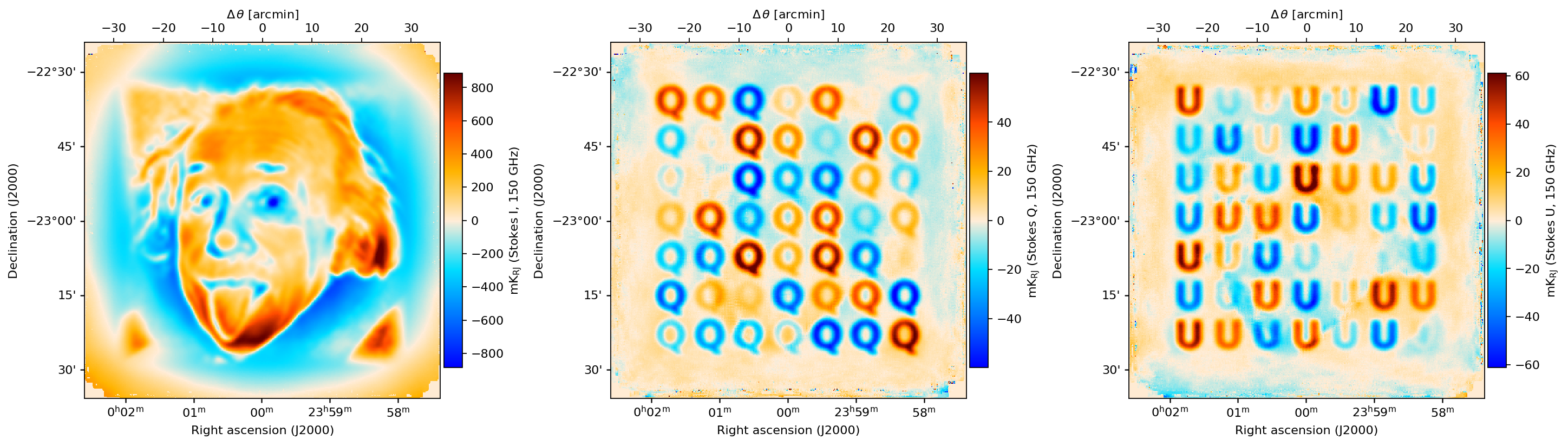
Note that we can’t see any of the circular polarization, since our instrument isn’t sensitive to it.