Simulating observations with MUSTANG-2
MUSTANG-2 is a bolometric array on the Green Bank Telescope. In this notebook we simulate an observation of the Crab Nebula (M1).
[1]:
import maria
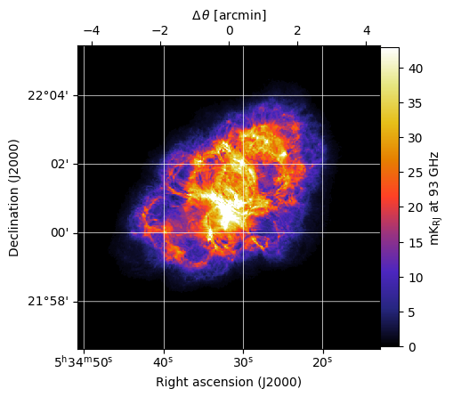
input_map = maria.map.get("maps/M1.h5").to("K_RJ")
input_map.data[input_map.weight < 0.2 * input_map.weight.max()] = 0
input_map.plot(slices="all")
print(input_map)
2026-06-05 13:48:53.947 INFO: Fetching https://github.com/thomaswmorris/maria-data/raw/master/maps/M1.h5
Downloading: 100%|██████████| 21.8M/21.8M [00:00<00:00, 187MB/s]
ProjectionMap:
  data(1, 3, 1205, 1187):
    min: -6.150e-02
    max: 5.613e-01
    units: K_RJ
    quantity: rayleigh_jeans_temperature
  stokes(1):
    components: ['I']
  nu(3):
    values: [149.8962 214.1375 272.5386] GHz
  eta(1205):
    height: 20.07’
    res: -1”
  xi(1187):
    width: 19.77’
    res: 1”
  frame: ra/dec
  center:
    ra: 05ʰ34ᵐ31.95ˢ
    dec: 22°00’52.16”
  beam(maj, min, psi): ragged
  memory: 34.33 MB
[2]:
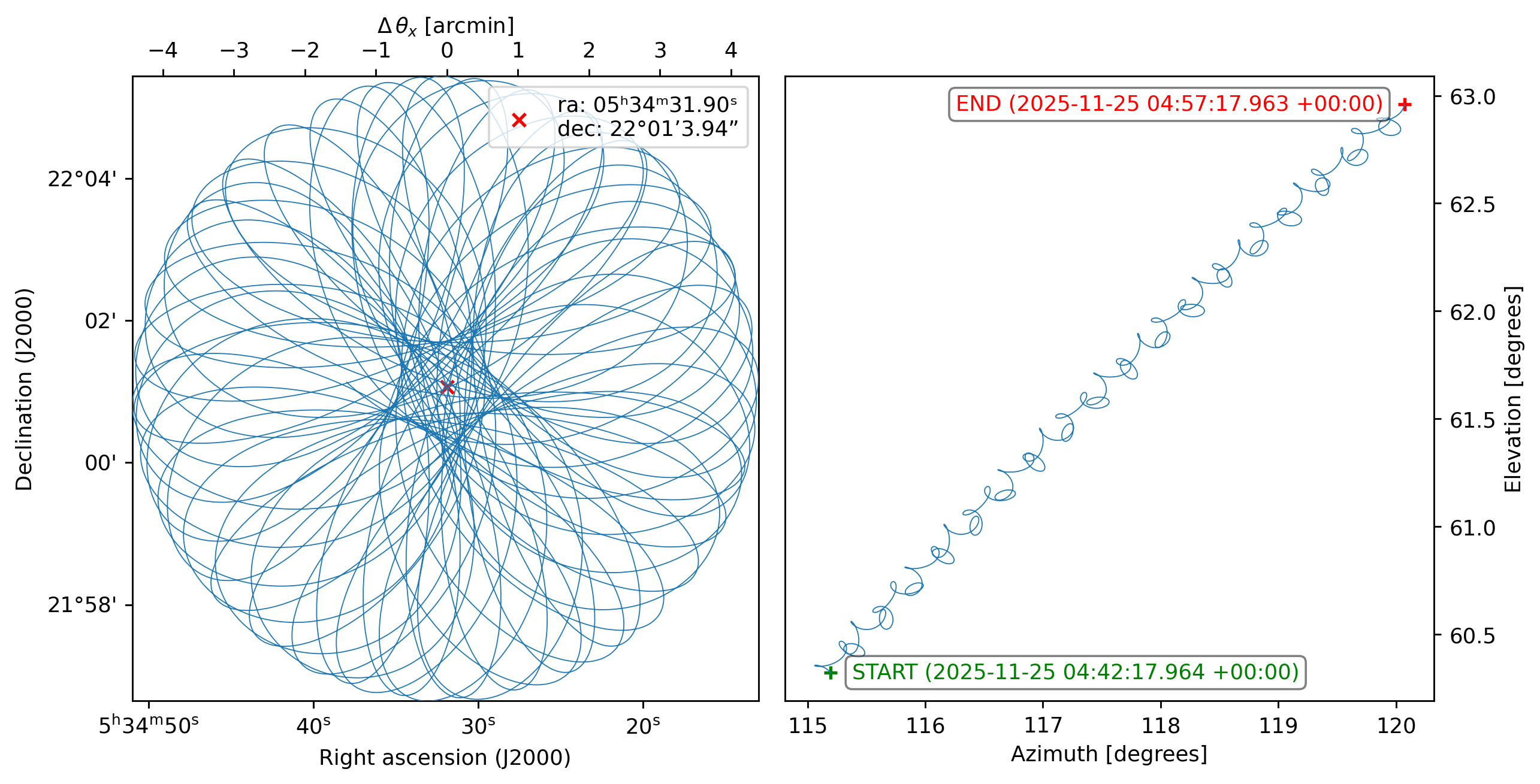
from maria import Planner

planner = Planner(target=input_map, site="green_bank", constraints={"el": (60, 90)})
plans = planner.generate_plans(total_duration=600, sample_rate=50)

plans[0].plot()
print(plans)
PlanList(1 plans, 600 s):
                           start_time duration    target(ra,dec)     center(az,el)
chunk
0      2026-06-05 16:02:07.274 +00:00    600 s  (83.63°, 22.02°)  (116.3°, 60.97°)
[3]:
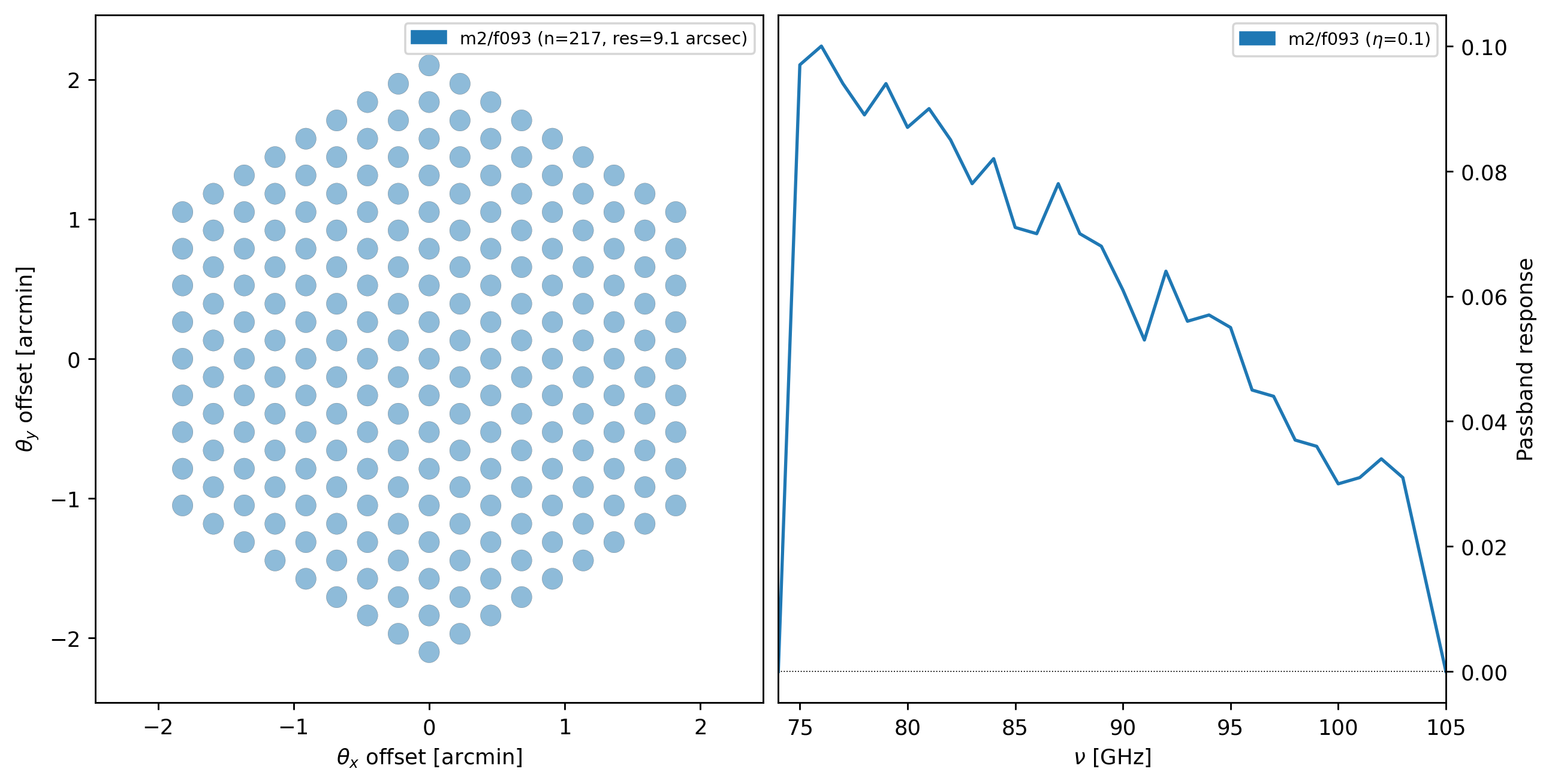
instrument = maria.get_instrument("MUSTANG-2")

print(instrument)
instrument.plot()
Instrument(1 array)
├ arrays:
│            n field_of_view max_baseline      bands polarized primary_size
│  array1  217          4.2’          0 m  [m2/f093]     False        100 m
│
└ bands:
         name     center      width    η      NEP         NET_RJ         NET_CMB    FWHM
   0  m2/f093  86.21 GHz  20.98 GHz  0.1  15 aW√s  571.1 uK_RJ√s  690.5 uK_CMB√s  9.133”
[4]:
sim = maria.Simulation(
    instrument,
    plans=plans,
    site="green_bank",
    map=input_map,
    atmosphere="2d",
)

print(sim)
2026-06-05 13:49:06.956 INFO: Fetching https://github.com/thomaswmorris/maria-data/raw/master/atmosphere/spectra/am/v3/green_bank.h5
Downloading: 100%|██████████| 22.0M/22.0M [00:00<00:00, 161MB/s]
2026-06-05 13:49:08.114 INFO: Fetching https://github.com/thomaswmorris/maria-data/raw/master/atmosphere/weather/era5/green_bank.h5
Downloading: 100%|██████████| 12.0M/12.0M [00:00<00:00, 152MB/s]
Constructing atmosphere: 100%|██████████| 8/8 [00:00<00:00, 11.57it/s]
Simulation
├ Instrument(1 array)
│ ├ arrays:
│ │            n field_of_view max_baseline      bands polarized primary_size
│ │  array1  217          4.2’          0 m  [m2/f093]     False        100 m
│ │
│ └ bands:
│          name     center      width    η      NEP         NET_RJ         NET_CMB    FWHM
│    0  m2/f093  86.21 GHz  20.98 GHz  0.1  15 aW√s  571.1 uK_RJ√s  690.5 uK_CMB√s  9.133”
├ Site:
│   region: green_bank
│   timezone: America/New_York
│   location:
│     longitude: 79°50’23.28” W
│     latitude:  38°25’59.16” N
│     altitude: 825 m
│   seasonal: True
│   diurnal: True
├ PlanList(1 plans, 600 s):
│                            start_time duration    target(ra,dec)     center(az,el)
│ chunk
│ 0      2026-06-05 16:02:07.274 +00:00    600 s  (83.63°, 22.02°)  (116.3°, 60.97°)
├ Atmosphere(8 processes with 8 layers):
│ ├ spectrum:
│ │   region: green_bank
│ └ weather:
│     region: green_bank
│     altitude: 825 m
│     time: Jun 5 12:07:07 -04:00
│     pwv[mean, rms]: (24.2 mm, 726.1 um)
└ ProjectionMap:
    data(1, 3, 1, 1205, 1187):
      min: -6.150e-02
      max: 5.613e-01
      units: K_RJ
      quantity: rayleigh_jeans_temperature
    stokes(1):
      components: ['I']
    nu(3):
      values: [149.8962 214.1375 272.5386] GHz
    t(1):
      values: [1.78066733e+09] s
    eta(1205):
      height: 20.07’
      res: -1”
    xi(1187):
      width: 19.77’
      res: 1”
    frame: ra/dec
    center:
      ra: 05ʰ34ᵐ31.95ˢ
      dec: 22°00’52.16”
    beam(maj, min, psi): ragged
    memory: 34.33 MB
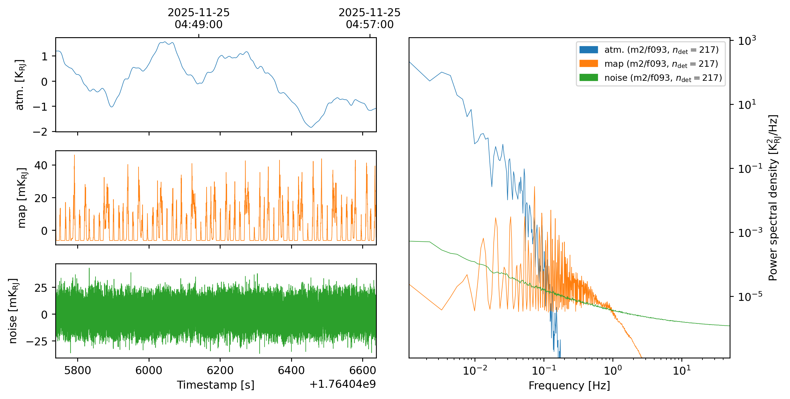
[5]:
tods = sim.run()
tods[0].plot()
2026-06-05 13:49:11.012 INFO: Simulating observation 1 of 1
Generating turbulence: 100%|██████████| 8/8 [00:00<00:00, 48.25it/s]
Sampling turbulence: 100%|██████████| 8/8 [00:03<00:00,  2.04it/s]
Computing atmospheric emission: 100%|██████████| 1/1 [00:00<00:00,  1.44it/s, band=m2/f093]
Sampling map: 100%|██████████| 1/1 [00:04<00:00,  4.45s/it, band=m2/f093, channel=(0 Hz, 182 GHz)]
Generating noise: 100%|██████████| 1/1 [00:00<00:00,  1.02it/s, band=m2/f093]
2026-06-05 13:49:25.015 INFO: Simulated observation 1 of 1 in 13.99 s
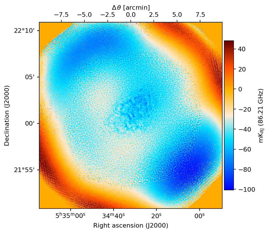
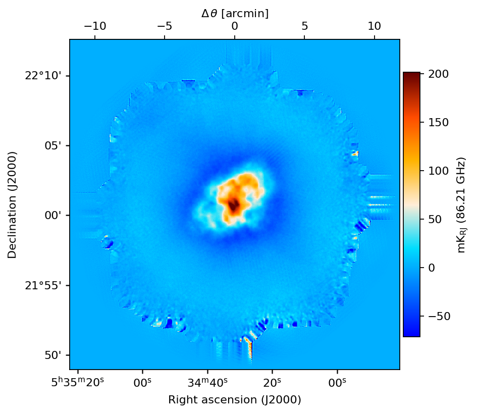
[6]:
from maria.mappers import MaximumLikelihoodMapper

mapper = MaximumLikelihoodMapper(
    units="K_RJ",
    tods=tods,
    resolution=input_map.resolution,
)

mapper.map.plot()
2026-06-05 13:49:29.520 INFO: Inferring center {'ra': '05ʰ34ᵐ32.21ˢ', 'dec': '22°00’56.33”'} for mapper
2026-06-05 13:49:29.532 INFO: Inferring mapper width 23.52’ for mapper from observation patch
2026-06-05 13:49:29.533 INFO: Inferring mapper height 23.52’ to match supplied width
2026-06-05 13:49:29.611 INFO: Inferring stokes parameters 'I' for mapper from detector sensitivities
Preprocessing TODs: 100%|██████████| 1/1 [00:02<00:00,  2.57s/it]
Computing pointing matrices: 100%|██████████| 1/1 [00:01<00:00,  1.60s/it]

[7]:
mapper.fit(epochs=1, steps_per_epoch=400, plot=True)
Updating noise model: 100%|██████████| 1/1 [00:01<00:00,  1.66s/it, tod=1/1]
Fitting map (epoch 1/1): 203it [04:08,  1.53s/it, alpha=0.353]2026-06-05 13:53:52.890 INFO: Finished conjugate gradient descent, terminating
Fitting map (epoch 1/1): 203it [04:10,  1.23s/it, alpha=0.353]
[8]:
from maria.mappers import compute_residual_map

residual_map = compute_residual_map(input_map[:, 0], mapper.map)
residual_map.plot()