Maximum likelihood mapmaking
[1]:
import maria
from maria.io import fetch
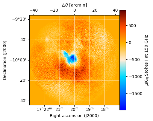
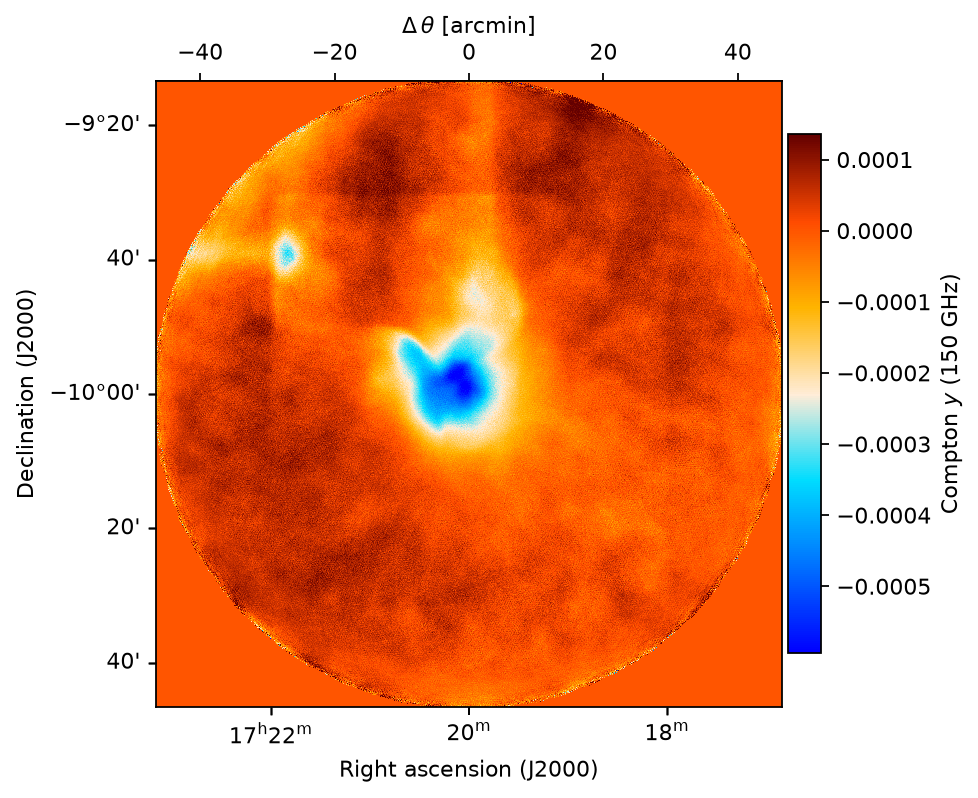
input_map = maria.map.get("maps/cluster2.fits", nu=150e9)
input_map.data *= 2e2
input_map.plot(cmap="cmb")
print(input_map)
2026-07-06 17:24:05.981 INFO: Fetching https://github.com/thomaswmorris/maria-data/raw/master/maps/cluster2.fits
Downloading: 100%|██████████| 4.20M/4.20M [00:00<00:00, 111MB/s]
ProjectionMap:
  data(1, 1024, 1024):
    min: -7.691e-04
    max: -1.001e-06
    units: compton_y
    quantity: compton_y
  nu(1):
    values: [150.] GHz
  eta(1024):
    height: 59.94’
    res: -3.516”
  xi(1024):
    width: 59.94’
    res: 3.516”
  frame: ra/dec
  center:
    ra: 17ʰ20ᵐ0.00ˢ
    dec: -10°00’0.00”
  beam(maj, min, psi): (0 rad, 0 rad, 0 rad)
  memory: 4.194 MB
[2]:
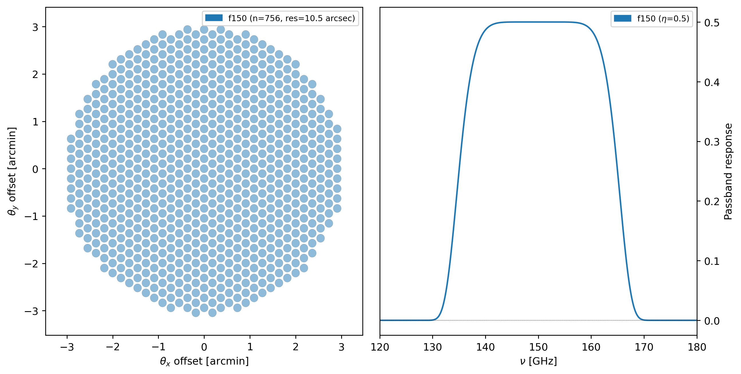
from maria.instrument import Band

f090 = Band(
    center=150e9,
    width=30e9,
    NET_RJ=10e-6,
    knee=5e1)

array = {"name": "my_custom_array",
         "field_of_view": 4 / 60,
         "primary_size": 30,
         "n": 121,
         "shape": "circle",
         "bands": [f090]}

instrument = maria.get_instrument(array=array)

print(instrument)
instrument.plot()
Instrument(1 array)
├ arrays:
│                     n field_of_view max_baseline   bands polarized primary_size
│  my_custom_array  121            4’          0 m  [f150]     False         30 m
│
└ bands:
      name   center   width    η         NEP      NET_RJ         NET_CMB   FWHM
   0  f150  150 GHz  30 GHz  0.5  2.204 aW√s  10 uK_RJ√s  17.33 uK_CMB√s  17.5”
[3]:
import numpy as np
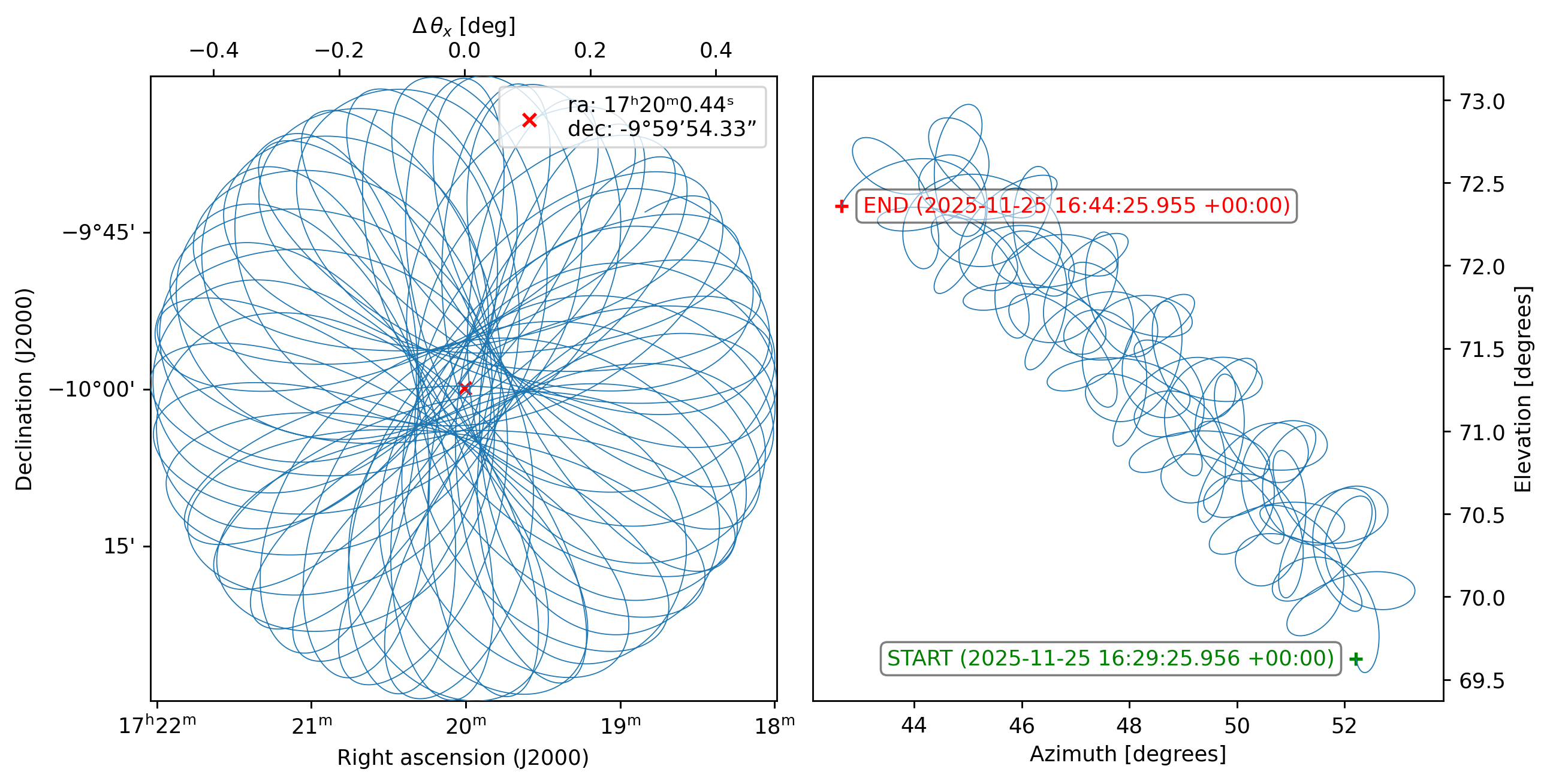
from maria import Planner
planner = Planner(start_time="2026-03-16T12:00:00",
target=input_map,
site="cerro_toco",
constraints={"el": (70, 90)})
plans = planner.generate_plans(
total_duration=2400,
max_chunk_duration=2400,
sample_rate=50,
scan_type="daisy",
scan_parameters={
"radius": 0.75 * input_map.width.deg,
"speed": 0.5,
})
plans[0].plot()
print(plans)
PlanList(1 plans, 2400 s):
                           start_time duration sample_rate target(ra,dec)     center(az,el)
chunk
0      2026-03-17 09:10:00.000 +00:00   2400 s       50 Hz   (260°, -10°)  (40.06°, 73.54°)
[4]:
sim = maria.Simulation(
    instrument,
    plans=plans,
    site="cerro_toco",
    map=input_map,
    atmosphere="2d",
    atmosphere_kwargs={"weather": {"pwv": 0.5}, "layers": {"boundaries": [0, 1000]}},
)

print(sim)
Initializing observations:   0%|          | 0/1 [00:00<?, ?it/s]
Constructing atmosphere:   0%|          | 0/1 [00:00<?, ?it/s]
Constructing atmosphere: 100%|██████████| 1/1 [00:00<00:00,  1.52it/s]
Initializing observations: 100%|██████████| 1/1 [00:03<00:00,  3.31s/it]
Simulation
├ Instrument(1 array)
│ ├ arrays:
│ │                     n field_of_view max_baseline   bands polarized primary_size
│ │  my_custom_array  121            4’          0 m  [f150]     False         30 m
│ │
│ └ bands:
│       name   center   width    η         NEP      NET_RJ         NET_CMB   FWHM
│    0  f150  150 GHz  30 GHz  0.5  2.204 aW√s  10 uK_RJ√s  17.33 uK_CMB√s  17.5”
├ Site:
│   region: chajnantor
│   timezone: America/Santiago
│   location:
│     longitude: 67°47’16.08” W
│     latitude:  22°57’30.96” S
│     altitude: 5.19 km
│   seasonal: True
│   diurnal: True
├ PlanList(1 plans, 2400 s):
│                            start_time duration sample_rate target(ra,dec)     center(az,el)
│ chunk
│ 0      2026-03-17 09:10:00.000 +00:00   2400 s       50 Hz   (260°, -10°)  (40.06°, 73.54°)
├ Atmosphere(1 processes with 1 layers):
│ ├ spectrum:
│ │   region: chajnantor
│ └ weather:
│     region: chajnantor
│     altitude: 5.19 km
│     time: Mar 17 06:29:59 -03:00
│     pwv[mean, rms]: (500 um, 15 um)
[5]:
tods = sim.run()
tods[0].plot()
2026-07-06 17:24:18.656 INFO: Simulating observation 1 of 1
Generating turbulence: 100%|██████████| 1/1 [00:00<00:00, 13.11it/s]
Sampling turbulence: 100%|██████████| 1/1 [00:01<00:00,  1.43s/it]
Computing atmospheric emission: 100%|██████████| 1/1 [00:01<00:00,  1.03s/it, band=f150]
Sampling source 'map': 100%|██████████| 1/1 [00:08<00:00,  8.56s/it, band=f150, message=Sampling channel (105 GHz, 195 GHz)]
Generating noise: 100%|██████████| 1/1 [00:01<00:00,  1.49s/it, band=f150]
2026-07-06 17:24:35.404 INFO: Simulated observation 1 of 1 in 16.74 s
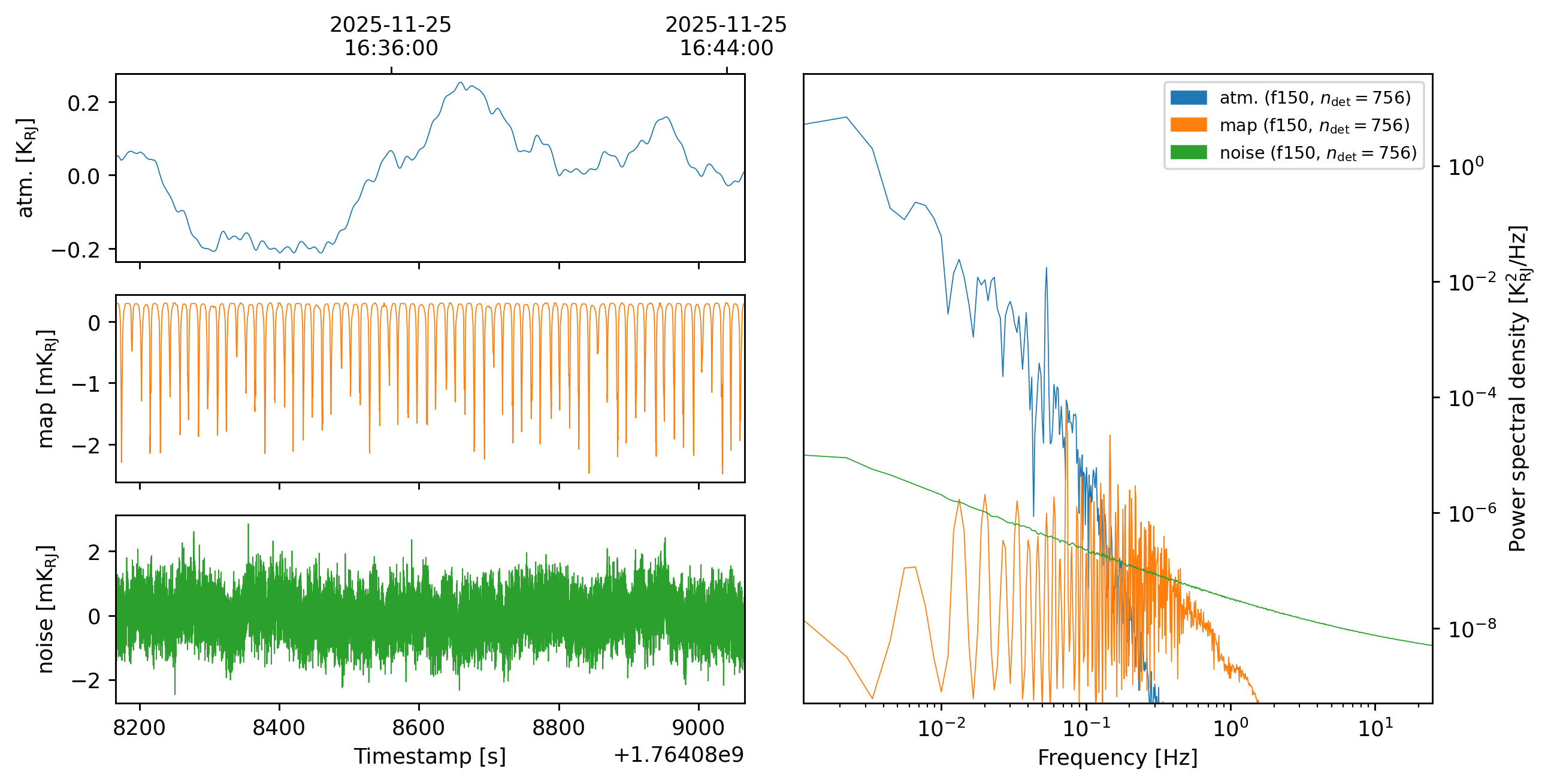
We can map the TOD with the MaximumLikelihoodMapper
[6]:
from maria.mapping import MaximumLikelihoodMapper

ml_mapper = MaximumLikelihoodMapper(tods=tods,
                                    tod_preprocessing={
                                        "remove_polynomial": {"time": 1, "elevation": 1},
                                    },
                                    init="bin",
                                    units="compton_y")
2026-07-06 17:24:40.116 INFO: Inferring resolution = 8.748” from detector FWHM
2026-07-06 17:24:42.393 INFO: Inferring center {'ra': '17ʰ19ᵐ59.95ˢ', 'dec': '-9°59’59.37”'} for mapper
2026-07-06 17:24:42.405 INFO: Inferring mapper width 1.554° for mapper from observation patch
2026-07-06 17:24:42.406 INFO: Inferring mapper height 1.554° to match supplied width
2026-07-06 17:24:49.056 INFO: Inferring stokes parameters 'I' for mapper from detector sensitivities
Preprocessing TODs: 100%|██████████| 1/1 [00:06<00:00,  6.41s/it]
Computing pointing matrices: 100%|██████████| 1/1 [00:03<00:00,  3.32s/it]
[ ]:
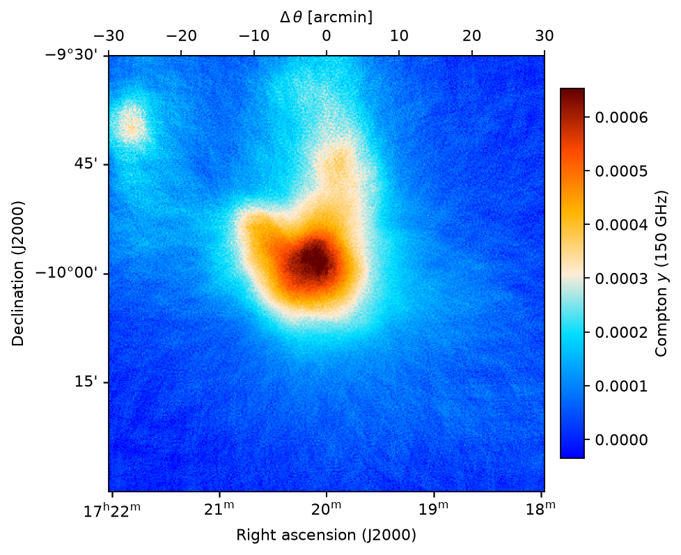
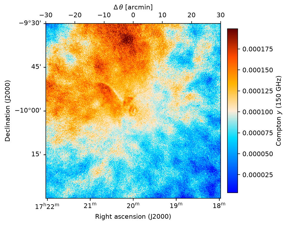
The initial solution is just a binning of the data, which has some noise artifacts and is missing some power (especially at large scales):
[7]:
from maria.mapping import compute_residual_map

print(ml_mapper.map)
ml_mapper.map.plot()

residual_map = compute_residual_map(input_map, ml_mapper.map)
residual_map.plot()
ProjectionMap:
  data(1, 639, 639):
    min: -5.391e-04
    max: 5.291e-04
    units: compton_y
    quantity: compton_y
  nu(1):
    values: [150.] GHz
  eta(639):
    height: 1.55°
    res: -8.748”
  xi(639):
    width: 1.55°
    res: 8.748”
  frame: ra/dec
  center:
    ra: 17ʰ19ᵐ59.95ˢ
    dec: -9°59’59.37”
  beam(maj, min, psi): (17.5”, 17.5”, 0 rad)
  memory: 3.267 MB
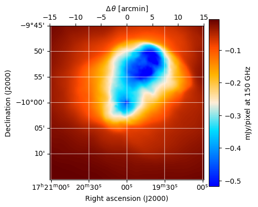
To improve the map, we build a noise model perform conjugate gradient descent to solve the mapmaking equation \(m = (P^\top N^{-1} P)^{-1} P^\top N^{-1} d\) where \(m\) is the map, \(P\) is the pointing matrix, \(N = \langle n \otimes n \rangle\) is the noise covariance, \(d = Pm + n\) is the data, and \(n\) is the noise.
[8]:
ml_mapper.fit(epochs=2, max_steps_per_epoch=50, plot=True)
Updating noise model: 100%|██████████| 1/1 [00:03<00:00,  3.91s/it, tod=1/1]
Fitting map (epoch 1/2): 50it [01:53,  2.28s/it, alpha=78]
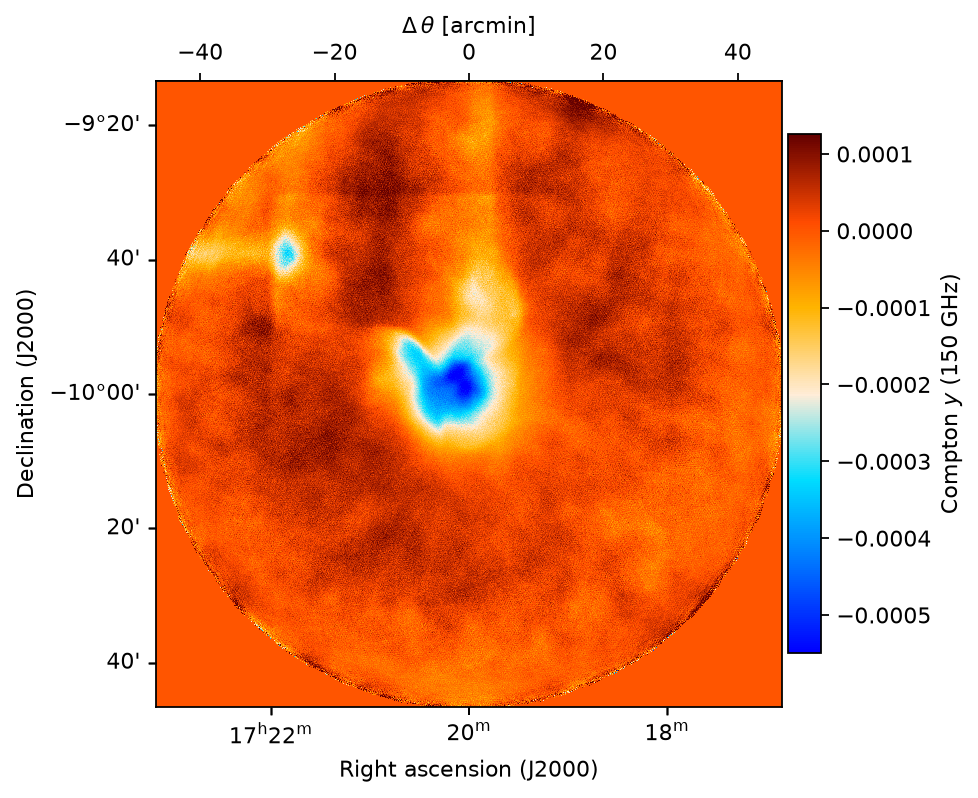
Updating noise model: 100%|██████████| 1/1 [00:03<00:00,  3.84s/it, tod=1/1]
Fitting map (epoch 2/2): 50it [01:53,  2.27s/it, alpha=78.6]
[9]:
from maria.mappers import compute_residual_map

residual_map = compute_residual_map(input_map, ml_mapper.map)
residual_map.plot()
and our inverse variance map looks like
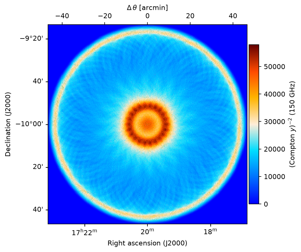
[10]:
ml_mapper.map.plot(attr="weight")